Introduction #

Continuing the path of learning about deep learning, I have been working on building a diffusion/flow matching models from scratch on and off for a while. My initial goal was to build a flow-matching or diffusion model for audio with mel-spectrograms inputs. However, after struggling with eyeballing generated melspectrogram to determine if it’s good or bad and the added complexity of dealing with melspectrogram to audio conversion, I decided to pivot to the image domain first to make sure I learn the diffusion modeling aspect properly before tackling audio. Specifically, I chose to go with with the classic celebrity datasets, allowing me to focus on the core mechanics of generation.

tl;dr In this blog post, I discuss building a flow matching image generator from scratch by following the papers Back to Basics: Let Denoising Generative Models Denoise. Python Notebook with full implementation is here

Flow Matching and Back to Basics Paper #

Flow matching and diffusion models is about building a model to generate images by progressively “cleaning” a noisy version of the image until it’s clean. Suppose x₀ represents pure noise, and x₁ represents clean image (our target), the model learns to progressively transform x₀ to x₁ via an equation simliar to

In most common formulations, models are trained to predict noise ϵ. In this framework, the model estimates the specific noise residual that was added to the data to reach the current state x(t) at timestep t. By calculating this predicted noise, we can iteratively move toward a cleaner image by “subtracting” the predicted noise at each step.

A recent paper that I came cross, Back to Basics, suggests learning is most effective when model focuses on data distribution rather than the noise distribution. Specifically, the paper suggested building a model to predict x (image) when given t and z, where z is a noisy version of the image and using the predicted velocity mean squared error (MSE) as the loss function.

This paper was eye opening for me because of how simple the formulation is and this is the implementation I converged upon. Straight from the paper, where JiT means Just Image Transformer

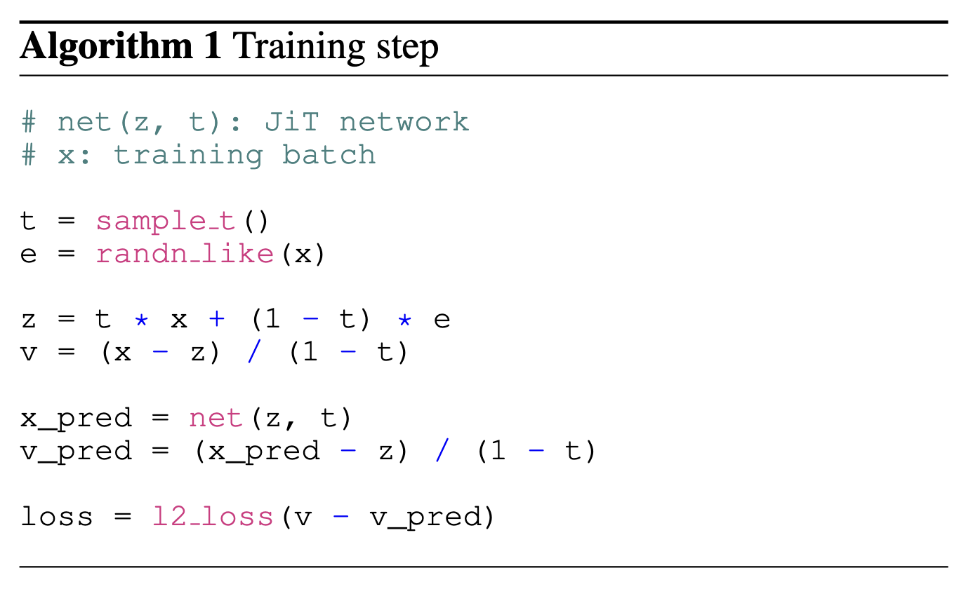
This algorithm will serve as the blueprint for the implementation in this post.

Highlight #

You can find the full notebook with dataloading, model, training loop and sampling here

Instead of copying and pasting the notebook verbatim in this blog, I will cover a high level overview and deep dive into a few areas I found interesting from building this project.

I used a standard transformer architecture with self attention, with some modern tweaks such as QK norm, SwiGLU activation, and RoPE embedding. As an experiment, I also tried using Derf instead of RMSNorm. The model generates 256x256x images.

Image to Patch Tokens #

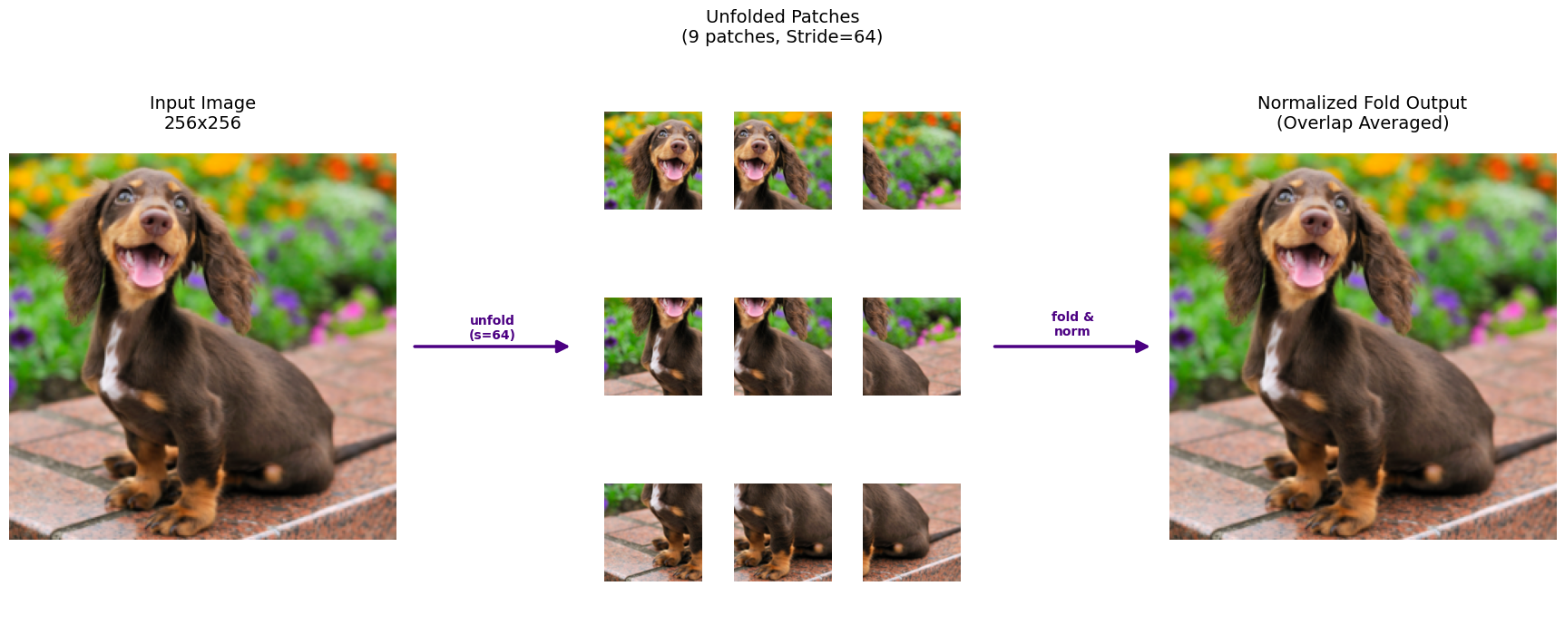
In order for the transformer to interact with images, which is represented as tensor of shape (C, H, W), we need to encode images into a sequence of “tokens”. Following standard literature practice, we will patchify the image; that is, we will chop the image into a sequence of small square images of size p and obtain a tensor of size (T, C’), where T = H * W // (p * p) and C' = p * p, assuming a stride of p, which results in no overlapping patches.

The patchify function is conveniently available inside torch.nn.functional module as

  F.unfold(
    img_tensor, 
    kernel_size=patch_size, 
    stride=patch_size)

The inverse function is

  folded_sum = F.fold(
    unfolded, 
    output_size=(H, W), 
    kernel_size=patch_size, 
    stride=stride)

Here is a screenshot showing visually what patchify looks like when stride is set to patch_size.

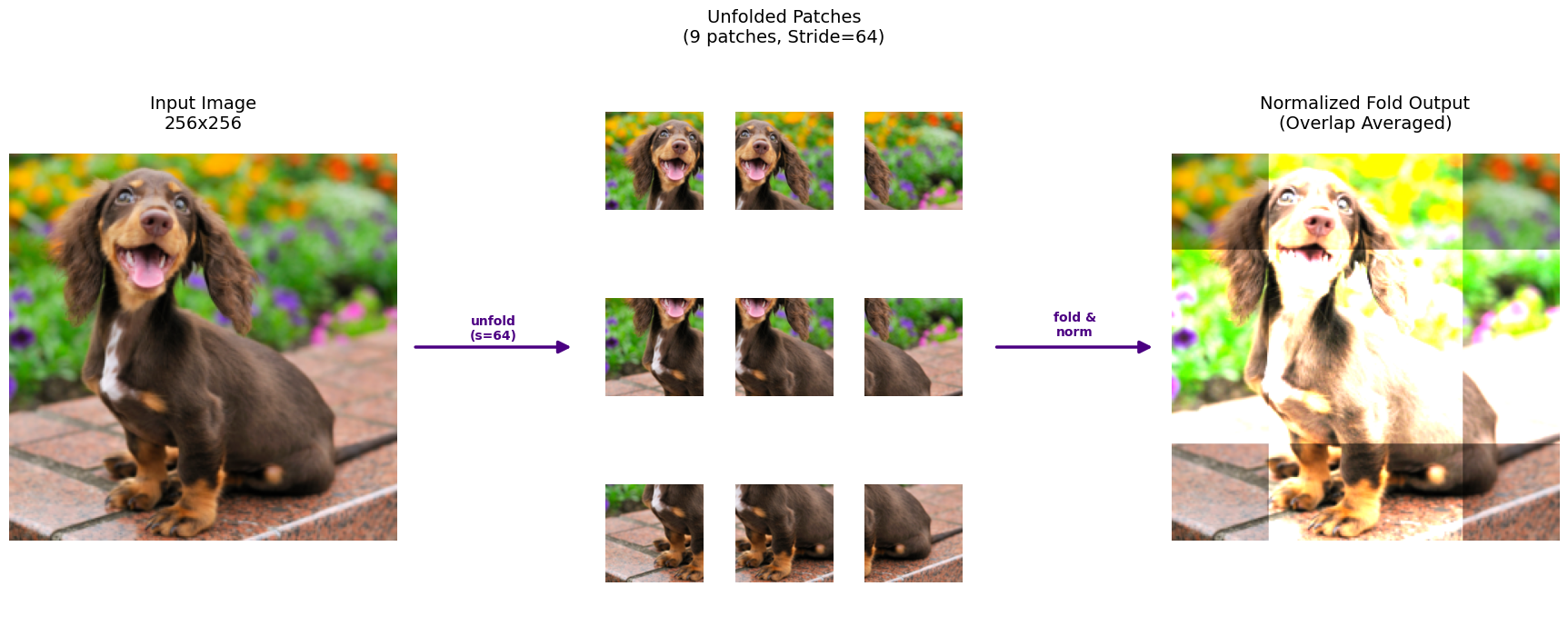
It can be beneficial to set stride lower than patch_size, say 50% or 25% to give our model more information. If our patches overlap (ie stride is less than patch), then when folding (turning patches back into image), it’s important to make sure to account for the overlap with a normalization mask.

    # Create a normalization mask (fold a tensor of ones)
    ones = torch.ones_like(unfolded)
    norm_mask = F.fold(
      ones, 
      output_size=(H, W), 
      kernel_size=patch_size, 
      stride=stride)
    folded_norm = folded_sum / norm_mask

If we didn’t normalize with the overlap mask, our image will be unnaturally bright in areas where patches overlap, as shown in the image below.

Noise Sampling Schedule #

In flow matching model, instead of feeding a clean image, we will feed a corrupted image. Let x be a clean image and z(t) be a corrupted image, where t represents time. z(0) is pure noise and z(1) equals x.

Following Back to Basics’ suggestion, we will make our transformer predict x (image space) and use velocity space (v) for our loss function.

That is, given t and corrupted input z,

Using x _predicted, loss function is

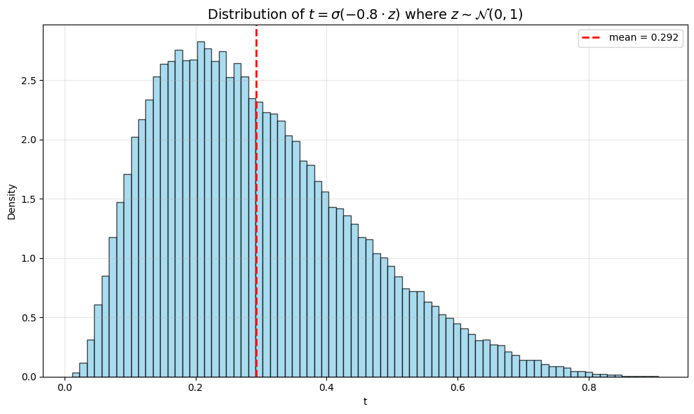
During training, we sample t to generate the corrupted images used for denoising. How we sample t is critical, as it dictates the specific distribution of corruption levels observed by the network. This is particularly important because of image redundancy: larger images contain more spatial information than smaller ones. For example, corrupting 42 pixels in a 64×64 image results in a ∼1% loss of information, whereas the same number of corrupted pixels in a 256×256 image represents a loss of only ∼0.06%.

This means as we scale up our model to generate higher resolution images, we have to adjust t sampling accordingly. Sample too many t close 1 biases our model to only see lightly corrupted images. I went with the suggested sampling schedule from Back to Basics for 256x256 images. For a reference paper on noise schedule, Simple Diffusion is a good resource.

import torch
import torch.nn.functional as F
import numpy as np

def sample_logit_t(dim, resolution=256, base_res=256, sig=0.8, mu_base=-0.8):
    """
    Adjusts the logit-normal sampling mean based on resolution.
    Shifts the distribution to higher noise for higher resolutions.
    """
    # 1. Calculate the resolution shift (from Simple Diffusion paper)
    # As resolution increases, we shift the mean to sample higher noise levels
    mu = mu_base - math.log(resolution/base_res)
    
    # 2. Sample from logit-normal distribution
    u_sample = torch.randn(dim) * sig + mu
    t = torch.sigmoid(u_sample)
    
    return t

A graph showing the distribution of t for the sampling schedule used in my training setup.

Solving ODE with Euler #

One of the core mechanisms of the Flow Matching algorithm is the need to iteratively solve an Ordinary Differential Equation (ODE). Specifically, we will leverage our flow matching model to derive a velocity field (position over time), and use that to nudge our image (position) step by step until we get a noise free version.

While many implementations use complex adaptive solvers, in keeping with the spirit from scratch as much as possible, I have chosen to go with implement Euler’s method.

The core idea is as follows: suppose you have a function x(t) and you know both its derivative dxdt and its value at a specific t. To estimate the value of X at new value t2, we can start from x(t), take a small step in the directions of the dxdt(t), arrive at new value x(t + epsilon). In equation form

In equation form

We can repeat this process until we arrive at t2 and get at an estimate for x(t2).

The smaller the epsilon, the better the approximateion and the smaller the error.

@torch.no_grad
def euler_method(y0, x0, x1, dfdx):
    x = x0
    x_tensor = torch.tensor(x).to(y0.device)
    
    y = y0
    B = y.shape[0]
    while x < x1:
        dfdx_val = dfdx(y, x_tensor.repeat(B))
        y = y + step_size * dfdx_val
        x += step_size
        x_tensor = torch.tensor(x).to(y0.device)
    return y

To verify the euler function is working correctly, here is a visualization of euler function approximating sine wave with different step sizes (the bigger the steps, the smaller the epislon)

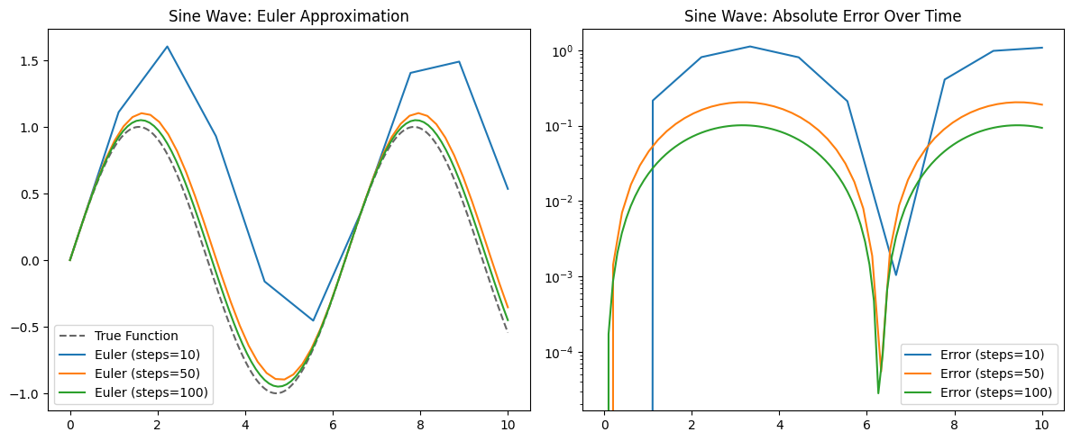
As we can see, while not perfect, with 100 steps, euler method matches sine wave shape very well.

Results #

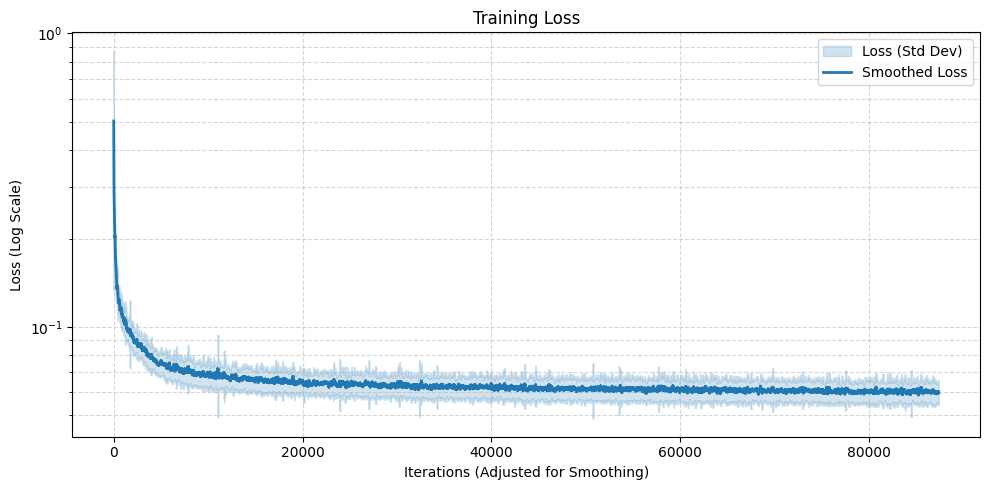
I ran the training loop on the full celebrity dataset using a 12-layer transformer (~114M params). With an embedding size of 768, patch_size=16, and stride=12, the model reached 100 epochs in about 6 hours on an RTX 5090.

Here are few selected samples of what the model can generate after this modest training

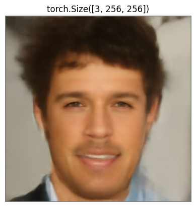
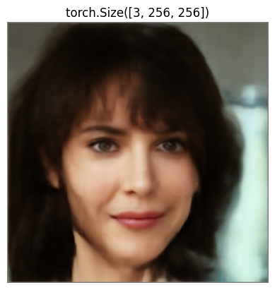
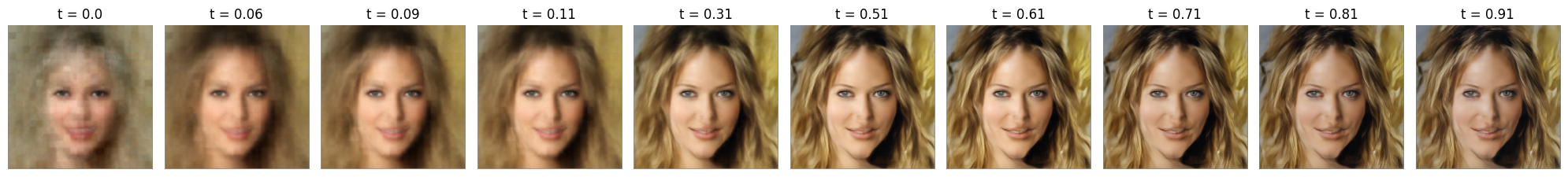
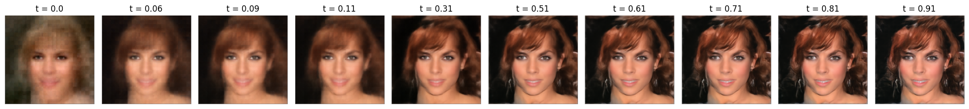
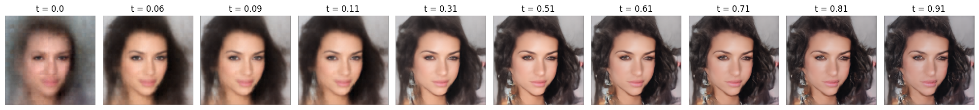
While far from perfect, these images demonstrate that model successfully learnt facial positions and the overlapping patches successfully mitigated grid like artifacts, a common failure mode I encountered during the course of this exercise.

Noticeable denoising artifacts appear at the high t end of the spectrum, likely due to the noise sampling schedule’s bias toward lower t values. This could be resolved with an adjusted noise schedule, which I will leave for future exploration.

Reflection #

I think it’s important to point out this learning path has been highly nonlinear. There were many debugging sessions (is rope implementation correct? is my attention implementation correct) and reading different papers to try to get to the essence of the flow matching algorithm.

In an era where a single prompt to a LLM can generate anything, one might ask: what is the point of spending all these time to write a blog to document the journey? For me, it boils down to the pure joy of building. It’s much like hiking - there is a deep, quiet satisfaction in setting a goal and seeing it through to the end, regardless of how many others have trekked the same path. Similarly, I find that writing these posts remains rewarding because it represents a mini milestone in my learning journey.