Overview #

After coming across Ha & Schmidhuber’s 2018 paper World Models earlier this year, I have been working on building a “tiny world model” on a clone of Chrome’s Dino game.

The final model is small: a variational autoencoder (VAE), a recurrent world model and a two-layer actor. Getting the three pieces to work together required many rounds of debugging. There were many mistakes along the way: plausible-looking images hid a broken latent representation, a weighted loss hid a data problem, and a controller kept improving in an imagined world while getting worse in the real one.

tl;dr I followed the V-M-C recipe from World Models on a clone of Chrome’s Dino game, but trained the controller from scratch with Group Relative Policy Optimization (GRPO). The controller learnt entirely inside the world model and transferred to the real game. The most important lesson was to give every component an independent, honest metric before trusting the full pipeline.

Background #

Mentioning a world model in 2026 might evoke systems such as Genie 3, GameNGen or WHAM: models that generate rich, interactive worlds from simple text descriptions. Those systems are impressive, but the core idea is much smaller.

A world model is a statistical model that predicts how a world changes. Given a representation of the current state and an action, it predicts a distribution over the next state:

M(s_t, a_t) -> P(s_(t+1), d_(t+1))

Here, M is the world model, s_t is the state at time step t, and a_t is the action taken at that step. The output is P, a probability distribution over the next state s_(t+1) and whether the game has ended, d_(t+1). A state can be the rendered frame itself or, as we will see later, a compressed representation of the frame.

Why predict a distribution instead of a single next state? Even a small game can have more than one valid future. Given the same Dino frame and the same action, a new obstacle may or may not spawn at the edge of the screen. M needs to assign probability to both outcomes.

In the original World Models paper, the authors split the problem into three components:

1. V, a VAE that compresses each frame into a latent representation.
2. M, a mixture density network recurrent neural network (MDN-RNN) that predicts the next latent and terminal state.
3. C, a small controller trained inside the world imagined by M.

They applied the recipe to CarRacing and Doom and optimized the controller with an evolutionary algorithm. I adapted the same recipe to a Dino game clone and, instead of using an evolutionary algorithm, used GRPO, a reinforcement learning algorithm, to train the controller.

The rest of the post will discuss each component in detail.

Tiny Dino World #

In case you are not familiar with Chrome’s Dino game, it is a simple side-scroller where the dino jumps over cacti and ducks under birds.

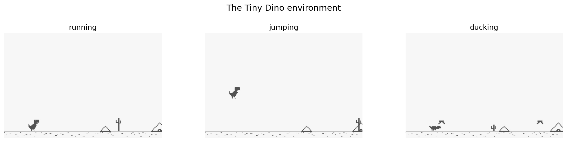
The world scrolls forward and procedurally spawns obstacles. The score increases while the dino stays alive and an episode ends when the dino hits an obstacle. It is simple, stochastic and, in theory, infinite, making it an ideal learning environment for a small world model.

I built the underlying environment as a deterministic 16 by 24 tile grid. Given the same seed and actions, it produces the same trajectory. Rendering is a pure function of the grid and frame tick, which made it possible to use the exact same pixels for training and playback.

Each rendered frame is a monochrome 512 by 768 image stored as a (512, 768, 3) RGB array. The action is one of three values: idle, jump or duck. I represent these as the one-hot vectors (1, 0, 0), (0, 1, 0) and (0, 0, 1) respectively. Finally, the environment has a boolean done state indicating that the dino collided with an obstacle.

I initially collected 10,000 transitions with a uniformly random policy. Each transition contains:

(s_t, a_t, r_t, d_(t+1), s_(t+1))

The subscript t means “at the current time step.” After taking action a_t in state s_t, the environment returns reward r_t, the next state s_(t+1), and d_(t+1) indicating whether that transition ended the episode.

I deliberately used a random policy for this first dataset. It is bad at the game, but that means the data contains both normal transitions and collisions. The 10,000 transitions included 206 collisions and covered both cactus sizes and low birds. A good heuristic policy almost never dies, which would give the done classifier very few positive examples to learn from.

Variational Autoencoder #

The first part of the recipe is a VAE that compresses a game frame into a compact latent space. I downsampled each frame by four, from (512, 768, 3) to (128, 192, 3), then passed it through a small residual convolutional encoder.

The encoder emits mu and logvar, the parameters of a diagonal Gaussian. A latent z is sampled with the reparameterization trick:

def reparameterize(mu, logvar):
    std = (0.5 * logvar).exp()
    epsilon = torch.randn_like(std)
    return mu + std * epsilon

The decoder performs the reverse operation, expanding the 128-value latent back into an image. The complete path is:

Image (3 x 128 x 192)
  -> Conv + [ResBlock x 2, Downsample] x 3
  -> mu, logvar (128 dim each)
  -> z = mu + sigma * epsilon
  -> Linear + [ResBlock x 2, Upsample] x 3
  -> sigmoid
  -> reconstructed image

The VAE objective combines reconstruction error with KL divergence:

L_VAE = reconstruction(x_hat, x)
        + beta * KL(q(z|x) || Normal(0, I))

The reconstruction term forces the latent to retain enough information to draw a Dino frame. The KL term pulls the posterior toward a standard Gaussian so that a random sample can also be decoded into a plausible frame. I used beta = 2.

The limiting cases helped me understand this objective. If beta is large, both mu and logvar are forced to be closer to 0 (sigma approaches 1), so the latent carries little information about the input. If beta is zero, the model becomes an ordinary autoencoder: reconstruction can be excellent, but arbitrary samples from a standard Gaussian are no longer guaranteed to decode cleanly.

MSE or BCE? #

I tried mean squared error (MSE) and binary cross entropy (BCE) for reconstruction. The renderer is almost binary: most pixels are either the off-white background or dark foreground. BCE therefore matches the data reasonably well as a Bernoulli likelihood and strongly penalizes a confident prediction on the wrong side of an edge. MSE corresponds to a fixed-variance Gaussian likelihood and made it easier for this model to settle on faint intermediate pixels.

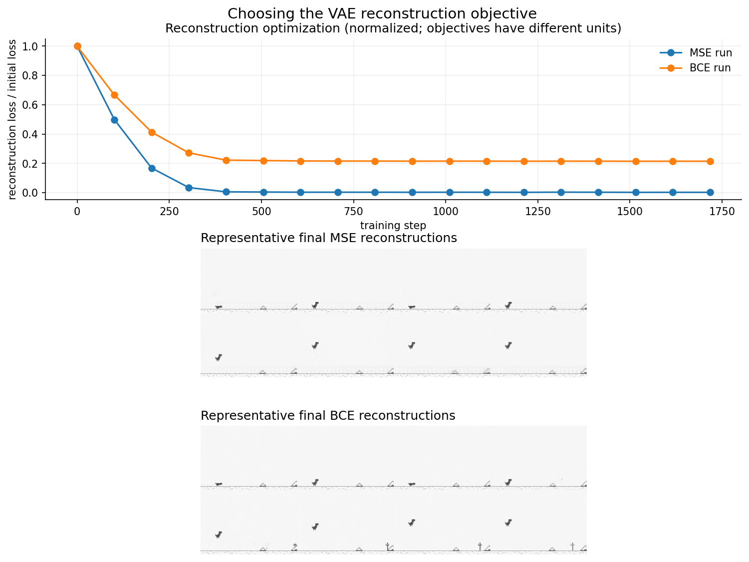
The BCE reconstructions were sharper in my runs, so I kept BCE. This was not a clean A/B test: the losses have different units and some architecture details changed between runs. While not a true apple to apple comparison, BCE converged faster and looked better so it’s the reconstruction loss I used.

As a final sanity check, I sampled z from a standard Gaussian and decoded it without an input image:

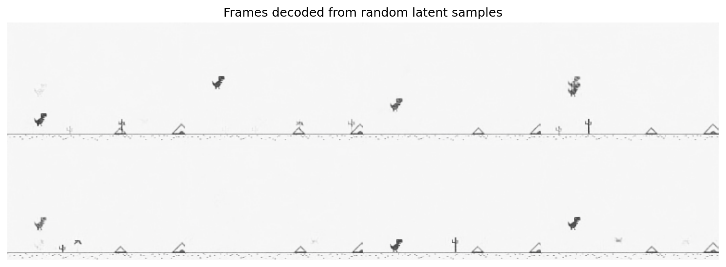
The samples are not perfect, but the ground, mountains, cacti, birds and dino are all recognizable. At this point I froze V and moved on to the world model.

World Model #

M needs to predict the next latent and whether the episode ends. I used an LSTM followed by a five-component mixture-density head and a separate binary done head:

class MdRnn(nn.Module):
    def __init__(self, z_dim=128, action_dim=3,
                 hidden_dim=512, n_mixtures=5):
        super().__init__()
        self.rnn = nn.LSTM(
            z_dim + action_dim, hidden_dim, batch_first=True
        )
        self.mdn = nn.Linear(
            hidden_dim, n_mixtures * (1 + 2 * z_dim)
        )
        self.done_head = nn.Linear(hidden_dim, 1)

    def forward(self, z, action, hidden=None):
        x = torch.cat([z, action], dim=-1)
        x, hidden = self.rnn(x, hidden)
        return self.mdn(x), hidden, self.done_head(x)

The output of self.mdn is one long vector containing the mixture logits, means and log standard deviations. The following helper splits that vector into the actual parameters:

import math

def get_mdn_params(mdn_output, n_mixtures=5, z_dim=128):
    B, T, _ = mdn_output.shape
    K = n_mixtures

    pi_logits = mdn_output[..., :K]
    mu = mdn_output[..., K:K + K*z_dim].reshape(B, T, K, z_dim)
    log_sigma = mdn_output[..., K + K*z_dim:].reshape(B, T, K, z_dim)

    pi = F.softmax(pi_logits, dim=-1)
    log_sigma = log_sigma.clamp(math.log(0.1), math.log(5.0))
    sigma = log_sigma.exp()
    return pi, mu, sigma

pi is the probability of selecting each of the five mixture components. Each component then has its own 128-dimensional mu and sigma. These are M’s candidate distributions for the next latent, not the mu and sigma produced by the VAE encoder. This lets M describe several possible next states instead of averaging every future into one point. The clamp keeps sigma between 0.1 and 5. Without it, unused mixture components grew standard deviations into the thousands while other components became overconfident.

State Representation: z or mu? #

Before training M, I had to choose which VAE output would represent a game state. The two obvious choices were the sampled latent z and the deterministic posterior mean mu. I started with z, and this choice caused most of the early world-model problems.

For the first latent dataset, I materialized one sampled z for every trajectory frame:

z_t = mu_t + sigma_t * epsilon_t

That single draw was saved to disk and M was trained to predict the next saved draw. At first the training looked encouraging. Loss went down and samples from M decoded into recognizable Dino frames.

I only realized something was wrong when I rolled M forward and tried to train the actor inside it. The frames had little temporal consistency and the actor collapsed because there was no stable sequence of states to learn from. The TensorBoard images looked good, but the model was not usable.

To investigate further, I added two metrics.

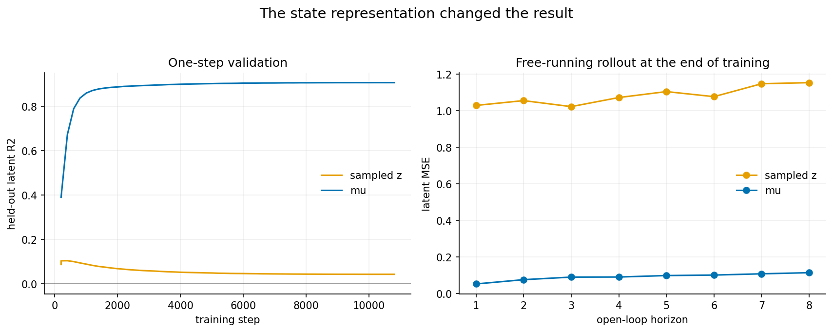
First, I added R-squared (R2), which measures how much of the variation in the true next latent is explained by M. R2=1 is a perfect prediction. R2=0 is no better than always predicting the average next latent. The sampled-z model finished at roughly R2=0.04, so it explained only about 4% of the held-out variation.

For a world model, this is a fundamental failure. The current z and action contained almost no usable information for predicting the saved next z. M could generate an individually plausible latent, but it could not preserve the relationship between one game state and the next. An actor trained on such rollouts sees a sequence of recognizable but mostly unrelated frames.

The second metric was open-loop MSE. I first gave the LSTM a few real states to initialize its hidden state. I then stopped supplying real latents and repeatedly fed M’s own prediction back as the next input. The sampled-z data had variance close to 1, so an MSE around 1 was roughly as bad as always predicting the average latent. The error stayed around 1 from horizon one through horizon eight.

Why did these bad predictions still decode into plausible frames? The VAE decoder had already learnt to turn samples from a broad standard Gaussian into something Dino-like. M only had to land somewhere in that broad region to produce a recognizable image. It had learnt the appearance of the game without learning how one frame leads to the next.

The VAE equation made the problem clear:

z = mu + sigma * epsilon,       epsilon ~ Normal(0, I)

Var(z) = Var(mu) + E[sigma^2]
       = 0.29    + 0.71
       ≈ 1.00

Var(mu)=0.29 is the variation in the deterministic posterior means across the encoded frames. E[sigma^2]=0.71 is the average variance added when sampling from each frame’s posterior. Since epsilon is independent for every frame, about 29% of the stored z variance came from the frame-dependent signal and 71% came from newly sampled noise.

On 171 consecutive frames, lag-1 correlation was 0.204 for mu but only 0.052 for sampled z. More decisively, an episode-split linear model could explain about 83% of next-mu variance but only about 7% of next-z variance.

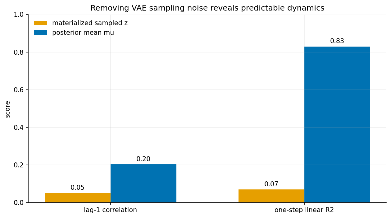
I had initially assumed that, because the VAE was trained one frame at a time and had no explicit time input, its latents did not need to be correlated across time. This was wrong. Consecutive game frames are visually related, so their deterministic encodings should also be related. mu preserved part of this relationship. Sampled z did not because every z also contained a new, independent noise term sigma * epsilon. That noise accounted for roughly 71% of z’s variance and overwhelmed the temporal relationship carried by mu.

Ha & Schmidhuber’s original implementation stored mu and logvar and resampled during RNN training. I had instead encoded each frame once and permanently stored that one sample in a dataset of only 10,000 frames. Unlike resampling, this permanently attached one random epsilon to every frame. I was asking M to predict the particular noise drawn during preprocessing.

I regenerated the dataset using mu for both the current and next state. M’s mixture head still models uncertainty in the game, such as whether an obstacle will spawn, but it no longer has to model noise introduced by the VAE encoder.

The effect was immediate. Validation R2 rose to 0.906, meaning M explained about 91% of held-out next-latent variation. Train and validation R2 stayed close to one another. Validation negative log likelihood (NLL), which measures how much probability M assigns to the true next latent, improved from -48 to about -249. Lower is better; for continuous probability densities, NLL can be negative. Open-loop MSE changed from roughly 1.03 -> 1.15 over eight steps to 0.052 -> 0.114.

The image below compares the two models more directly. The left column is M trained on sampled z; the right column is M trained on mu. Within each column, the top panel contains the actual next frames and the bottom panel contains M’s predictions for those same examples.

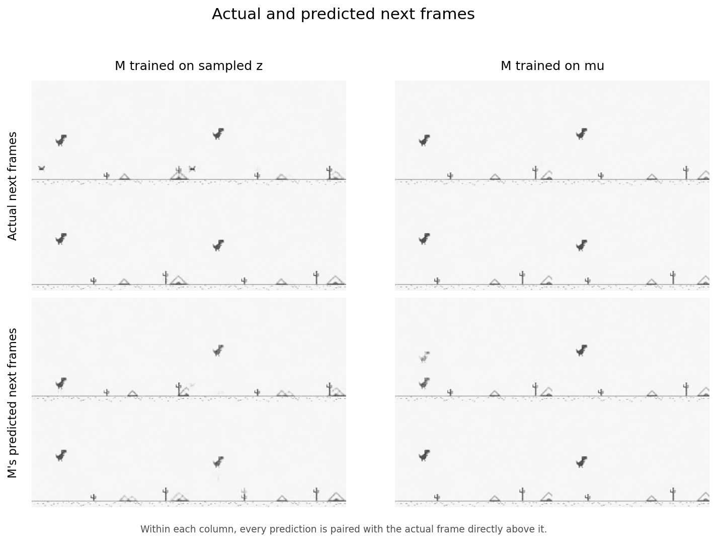
The sampled-z predictions still look like the game, but details from the actual next frames are missing or misplaced. The mu predictions track the dino and obstacle positions much more closely.

done Prediction #

The next issue was the done head. In the original 10,000-transition dataset, only 206 transitions were terminal. The validation windows contained just 19 positive examples.

At first I tried the standard class-imbalance fix: pos_weight ~= negative / positive in binary cross entropy. Recall reached 1.0, but precision was only 0.11. The model predicted too many collisions and was badly calibrated. That matters when training C in the dream: a false terminal prediction cuts off a trajectory and changes its reward.

I started exploring threshold calibration, then realized I was working around the wrong problem. If the concern was insufficient terminal data, the clean fix was to collect more terminal data.

Because collisions are rare, accuracy is not very useful: a model that always predicts “not done” would be more than 99% accurate. I tracked precision, recall, F1 and area under the precision-recall curve (AUPRC) instead. Precision asks how often a predicted collision is correct; recall asks how many real collisions the model catches. F1 is their harmonic mean. AUPRC summarizes the precision/recall tradeoff over all possible decision thresholds; for a random classifier, it is roughly the positive-example rate.

I expanded training to 50,000 transitions and validation to 5,000, giving the model 1,106 and 115 collision examples respectively. With enough positives, I removed the large class weight and trained with plain BCE. Held-out AUPRC reached 0.991; at P(done) > 0.5, precision was 1.0 and recall was 0.991.

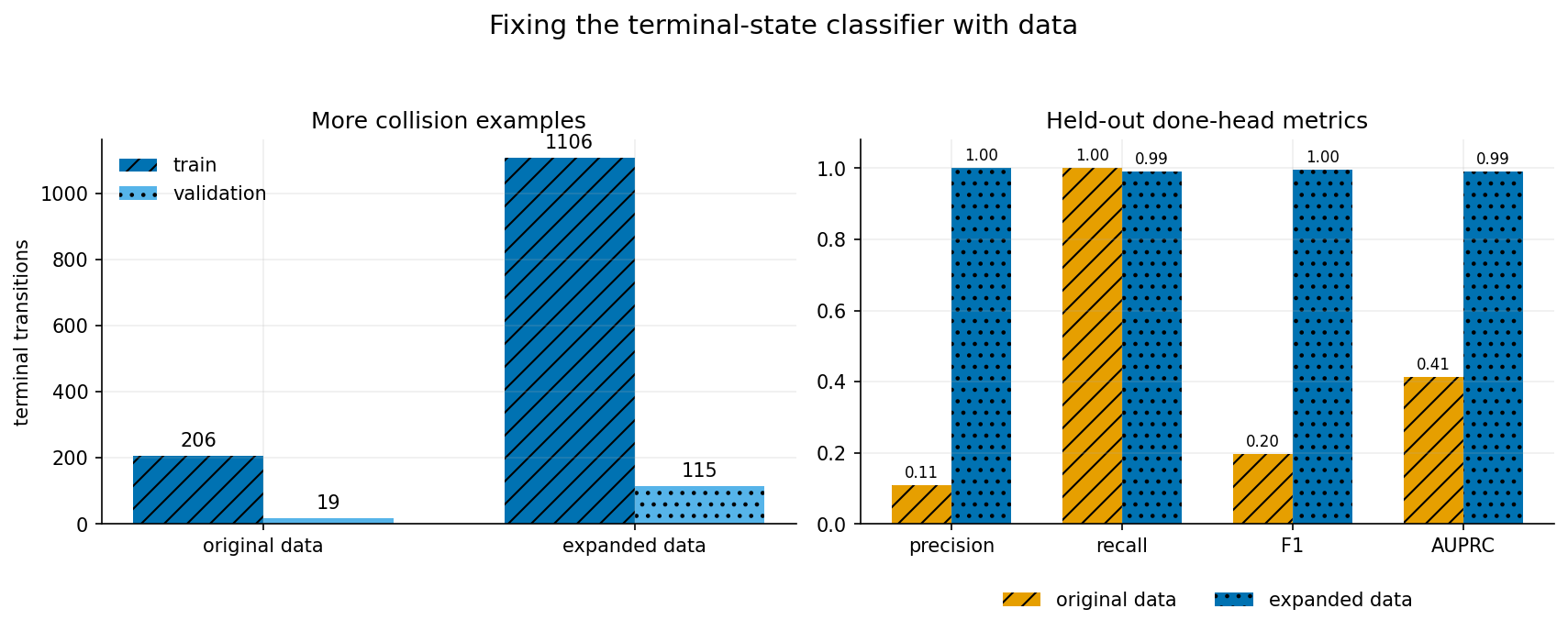
In this case, collecting better data was much more effective than tuning loss weights and classification thresholds.

Exposure Bias #

The initial RNN was trained with teacher forcing: at every position it received the real mu_t and predicted mu_(t+1). During a dream, however, the next input is its own previous prediction. Small errors move the model onto states it never saw during training, and those errors compound. This train/inference mismatch is called exposure bias.

To quantify the exposure bias, I warmed up the LSTM on four real states, then ran M in a free-running or open-loop mode for eight steps: after the warmup, each predicted latent became the input to the next step. I measured the error at each horizon.

I tried two corrections:

1. Add Gaussian noise to training inputs while keeping targets clean, teaching M to recover from a slightly wrong input.
2. Unroll M during training, feed its own prediction back, and backpropagate through the consequences.

The second method looks roughly like this:

prev = None
for t in range(sequence_length):
    z_in = z_true[:, t:t+1] if prev is None else prev
    mdn, hidden, done = model(z_in, action[:, t:t+1], hidden)
    pi, mu, sigma = get_mdn_params(mdn)

    loss = loss + mdn_nll(pi, mu, sigma, z_next[:, t:t+1])
    prev = mixture_mean(pi, mu)  # not detached: BPTT through rollout

Starting training with an eight-step free-running rollout is unstable because the model’s early predictions are poor and each bad prediction becomes the next input. To mitigate this, I tried curriculum training: pure teacher forcing, then free-run only the last K=2, K=4 and K=8 positions. The input-noise experiment flattened the error curve but raised the entire curve. Direct rollout training helped modestly at K=2, reducing eight-step MSE from 0.101 to 0.087; longer K=4 and K=8 stages did not continue the improvement. As the curriculum moved to four and then eight free-running steps, eight-step MSE climbed back to approximately 0.101. The best checkpoint was therefore in the K=2 stage, not at the end of training. To understand why the longer curriculum did not help, I looked more closely at what long-horizon MSE was measuring.

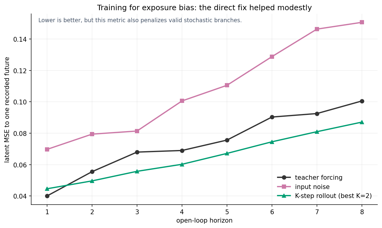
I had been interpreting any increase in long-horizon MSE as model degradation. That was too simple. Obstacle spawning is stochastic. From the same state, several future cactus layouts can all be valid. MSE against one recorded trajectory penalizes a valid alternate branch.

To validate this, I decoded several samples from the same starting state:

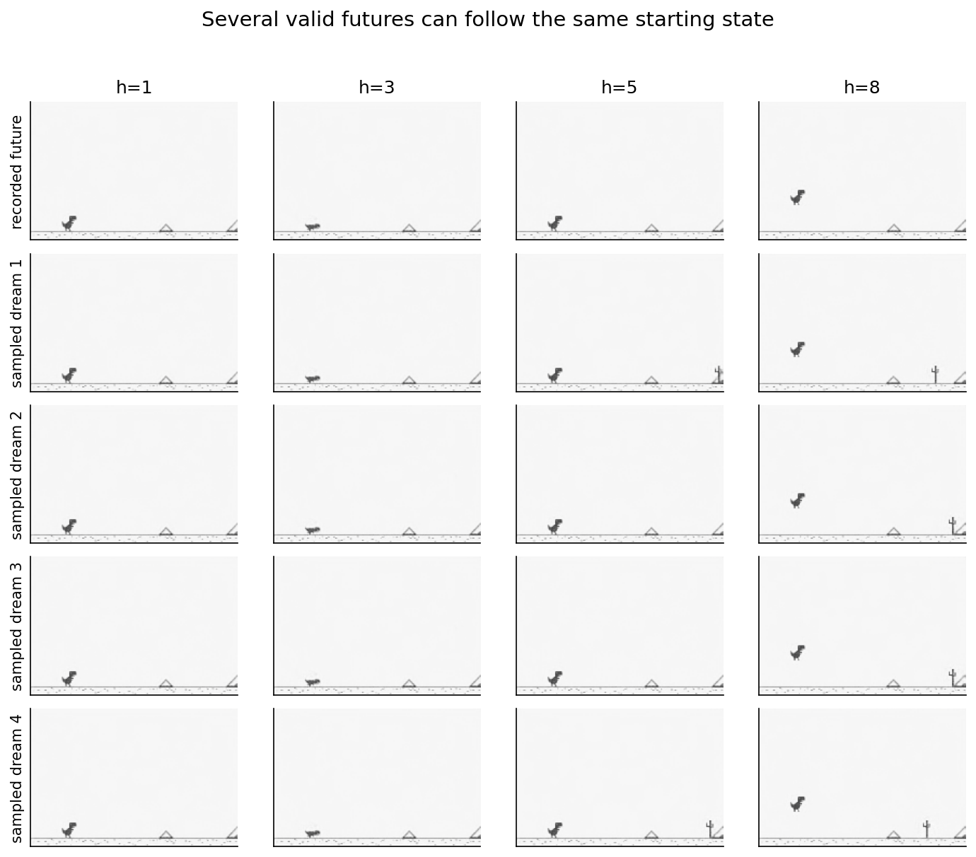
The dreams agree early, then branch into different obstacle configurations while remaining recognizable. On a representative batch, the decoded-frame Structural Similarity Index Measure (SSIM) stayed near 1.0 even while latent MSE rose. SSIM compares local brightness, contrast and image structure; 1.0 means two images are identical. The mostly blank background makes SSIM overly generous for this game, so I use it in combination with the filmstrip and rollout MSE.

I kept MSE as a useful metric, but stopped treating distance to one recorded future as the complete evaluation of a stochastic model.

Actor Model #

With V and M frozen, the last component is the controller. It is deliberately small:

class Actor(nn.Module):
    def __init__(self):
        super().__init__()
        self.net = nn.Sequential(
            nn.Linear(128, 128),
            nn.Tanh(),
            nn.Linear(128, 3),
        )

    def forward(self, z):
        return self.net(z)  # logits for idle, jump, duck

Training in a Dream #

A dream starts from a real encoded frame. The actor chooses an action, M predicts the next latent and done, and that predicted latent is fed back to the actor. The reward is one for every step entered alive, so maximizing return means surviving as long as possible.

Training inside M means the loop no longer needs to render pixels or step the real Python environment. Once M has learnt the dynamics, the actor can generate many training episodes cheaply in imagination.

The reward is non-differentiable through the sampled action and terminal decision. The original paper used an evolutionary algorithm. I took this opportunity to learn and apply GRPO, introduced in DeepSeekMath.

For each starting latent, I sampled a group of eight rollouts. A trajectory’s advantage is its return relative to the other rollouts from the same start:

batch_size, horizon = rewards.shape
returns = rewards.sum(dim=1)
grouped = returns.view(n_starts, group_size)

advantage = grouped - grouped.mean(dim=1, keepdim=True)
advantage = advantage / (grouped.std(dim=1, keepdim=True) + 1e-8)
advantage_t = advantage.reshape(batch_size).unsqueeze(1).expand(-1, horizon)

There is no critic. If one rollout survives longer than its siblings, the actions in that rollout receive positive advantage; shorter rollouts receive negative advantage.

I reused each rollout for four gradient epochs. After the first update, the data is technically stale because it was sampled by the old policy. The PPO-style likelihood ratio and clipping keep those repeated updates bounded:

ratio = torch.exp(new_logprob - old_logprob)
surrogate = torch.minimum(
    ratio * advantage_t,
    torch.clamp(ratio, 1 - clip_eps, 1 + clip_eps) * advantage_t,
)
loss = -(surrogate * alive_mask).sum() / alive_mask.sum()
loss = loss - entropy_coef * entropy

alive_mask prevents padded steps after death from affecting the gradient. I tracked approximate KL, clip fraction, entropy, gradient norm and action fractions to make sure the optimizer itself remained healthy.

Dream vs. Reality #

For the final run, each update contained 32 starting states, eight rollouts per state and a maximum dream horizon of 256. Every 25 updates, I evaluated the actor in the real DinoEnv over 20 fixed seeds.

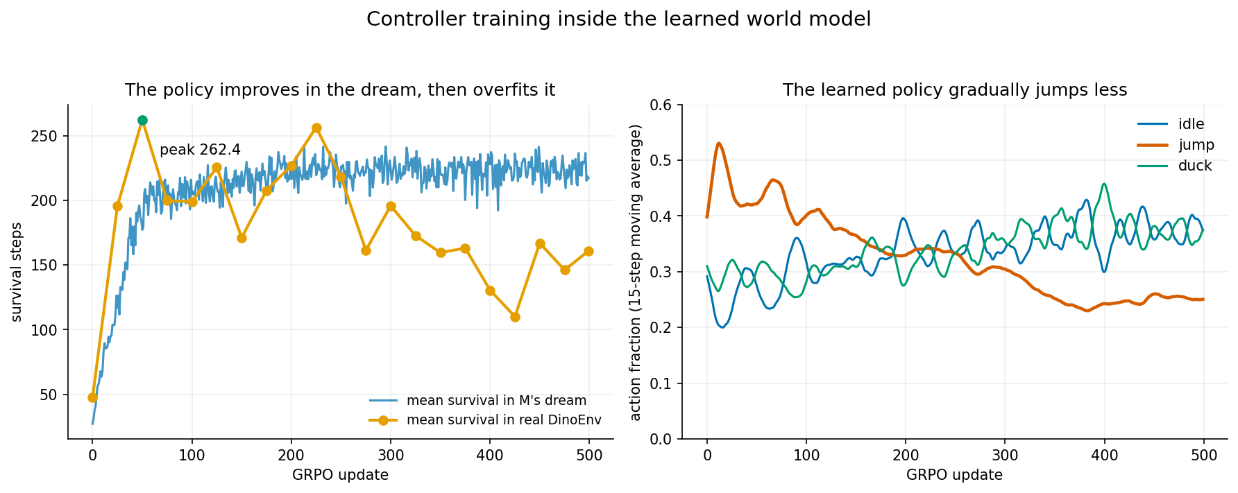
At the first evaluation, the actor survived an average of 47.6 real steps. After 25 GRPO updates it survived 195.7, and at update 50 it peaked at 262.4. The world model was providing a genuinely useful training signal.

Training longer was not better. Dream return remained around 220 to 240, while real survival eventually fell to 161.0. At the same time, the fraction of jump actions gradually dropped toward 0.25. The policy had found behavior that M considered safe but the real environment did not.

This is model exploitation: C becomes better at the learned world than at the world we care about. Approximate KL and clip fraction remained small, entropy did not collapse and gradients were stable. GRPO was doing its job; its objective had become a poor proxy for reality.

This means I should select the actor checkpoint using real-environment survival, not dream return. Other defenses would be to make dreams more stochastic, penalize disagreement between an ensemble of world models, or periodically collect trajectories from the current actor and refresh M on the states it now visits.

Voila! #

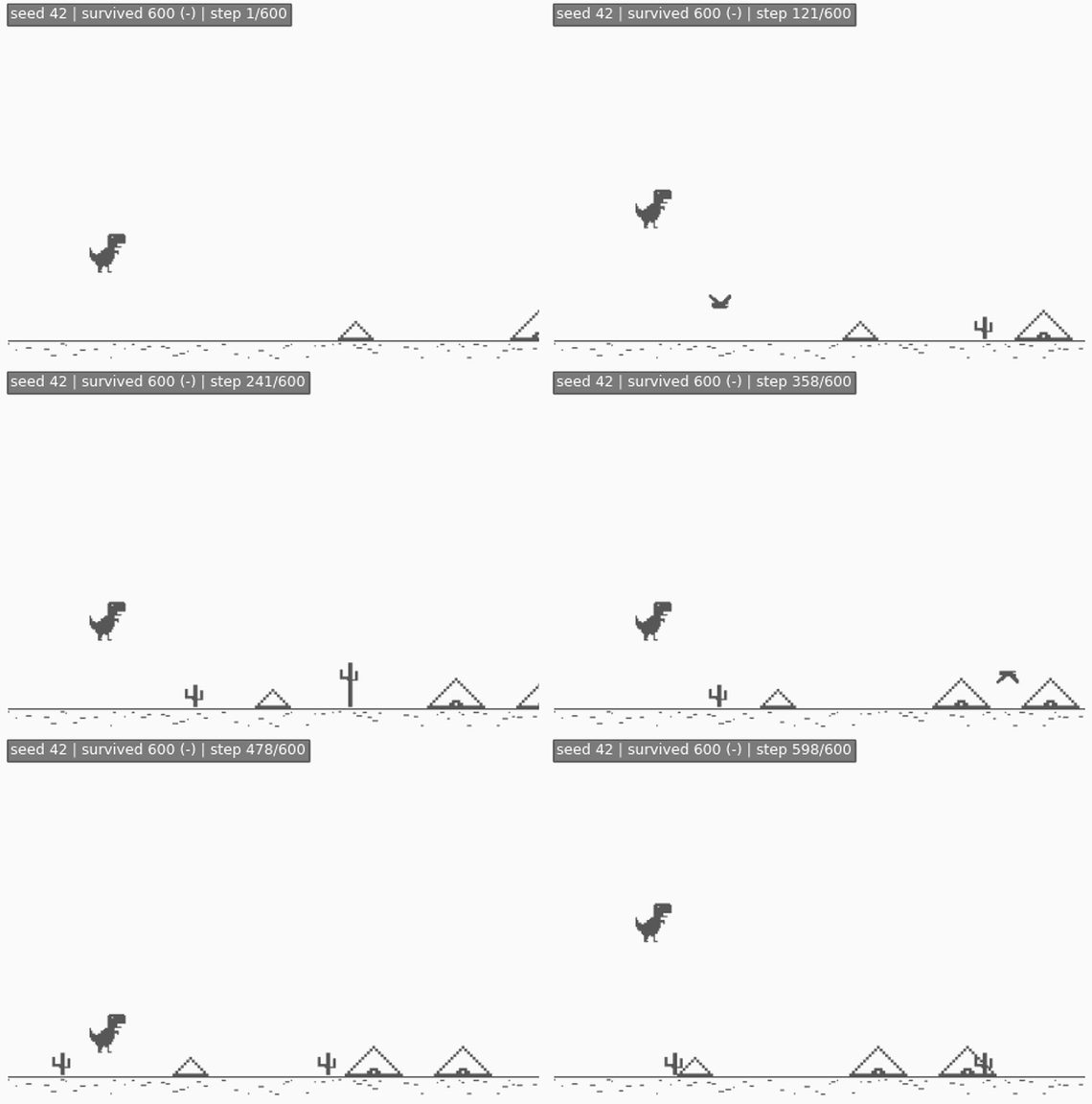
Putting everything together, here is the trained actor running against the real environment. While one good run is not a replacement for the multi-seed result above, watching a controller trained entirely in M’s dreams make the correct jump and duck decisions in the real environment shows that the complete V-M-C pipeline works end to end.

Conclusion #

The most important lesson from this project was not a particular architecture. It was the need to define what success means for every component before composing them.

• For V, reconstruction and random samples both mattered.
• For M, held-out latent R2, NLL and open-loop rollouts mattered; a nice decoded frame did not.
• For done, AUPRC, precision and recall mattered more than BCE.
• For C, real-environment survival was the metric; dream return alone eventually rewarded exploitation.

The project also helped me understand the difference between representing a distribution and selecting one outcome. I first encountered this in the VAE: mu and logvar describe a distribution around each frame rather than one fixed point, and the decoder must handle samples from that distribution. This posterior describes a neighborhood around one observed frame. M’s distribution serves a different purpose: it assigns probability to several possible future states.

C has a different objective. It searches for one sequence of actions with high reward. M needs to cover the plausible future modes, while C is mode seeking. Given enough optimization, C will seek not only good behavior but also any error in M that looks rewarding.

I think it is important to point out that this learning path was highly nonlinear. I first blamed the recurrent model when the real problem was VAE sampling noise. I tried calibrating a classifier when the real fix was more collision data. I treated long-horizon MSE as ground truth until visualizing valid branches. I also celebrated rising dream return before checking that the actor was getting worse in reality.

This has been a highly rewarding exercise. I can now trace the complete V-M-C path: V compresses pixels into a latent distribution, M predicts how that distribution evolves, and C learns inside the predicted future. More importantly, I learnt where each component can quietly fail and which metrics make those failures visible.

References #

• David Ha and Jürgen Schmidhuber, World Models, 2018.
• Zhihong Shao et al., DeepSeekMath: Pushing the Limits of Mathematical Reasoning in Open Language Models, 2024.
• Samy Bengio et al., Scheduled Sampling for Sequence Prediction with Recurrent Neural Networks, 2015.
• Dani Valevski et al., Diffusion Models Are Real-Time Game Engines, 2024.
• Google DeepMind, Genie 3: A New Frontier for World Models, 2025.
• Anssi Kanervisto et al., World and Human Action Models towards gameplay ideation, 2025.